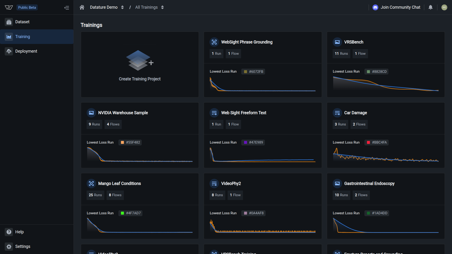
Training Metrics

The Metrics tab in Datature Vi shows quantitative measurements tracked throughout a training run. It displays loss curves, task-specific evaluation metrics, and the hyperparameters used for that run. For a plain-language introduction to these metrics, see How Do I Evaluate My Model?.

1

Open your training project

Go to Training in the sidebar and click the project containing the run you want to review.

Next →

You should see

Your metrics review is complete when you see both loss curves converging and evaluation scores stabilizing, indicating the model has finished learning.

Loss charts

Loss measures how far the model's predictions are from the ground truth. Lower loss indicates better alignment with training data.

Loss charts use two curve colors:

• Orange curves: training losses recorded at every training step (more granular)
• Blue curves: validation losses and metrics recorded at every evaluation interval (less granular)

Total loss

Total loss is the primary training metric. It shows overall model error over time.

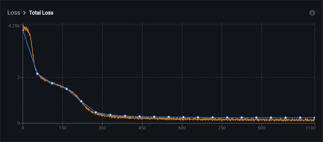
What to look for:

• Steady decrease: Model is learning
• Plateau at a low value: Model has converged
• Sudden spikes: May indicate learning rate issues or data quality problems
• No decrease: Model is not learning; check hyperparameters or dataset quality

What the loss numbers mean

Loss values depend on your model architecture and task. Rough reference ranges:

• Starting loss: typically 2.0 to 6.0 for untrained models
• Good final loss: 0.5 to 1.5 for well-trained models
• Excellent final loss: below 0.5 for high-quality datasets

Compare loss across runs for the same model and dataset. Different architectures have different loss scales, so absolute values are not directly comparable across model types.

Common loss curve patterns

Normal training: Both orange (training) and blue (validation) curves decrease together. The curves stay close throughout, which means the model is learning patterns that generalize to unseen data.

Underfitting: Both curves show little or no decrease and plateau at high values. The model has not learned enough from the data. Try training longer, using a larger model, or increasing the learning rate.

Overfitting: Orange (training) loss keeps decreasing while blue (validation) loss plateaus or increases. The gap between the two curves widens. The model is memorizing training data. See Understanding overfitting below for fixes.

Evaluation metrics

Evaluation metrics measure how well your model performs on specific tasks. Which metrics appear depends on your task type:

• Bounding box metrics: for phrase grounding tasks
• Text generation metrics: for visual question answering tasks

Bounding box metrics

These metrics apply to phrase grounding tasks and evaluate object detection quality.

When an image has many predicted and many ground-truth boxes, Datature Vi pairs them with Hungarian matching on pairwise IoU before counting matches. Each ground-truth box pairs with at most one prediction (and vice versa), which keeps precision, recall, and F1 interpretable in crowded scenes. A pair counts as a true positive for those metrics when its IoU meets the 0.5 threshold described below.

F1 score

F1 balances two things: how many of the model's predictions were correct (precision) and how many real objects the model found (recall). A high F1 means the model finds most objects without drawing too many wrong boxes.

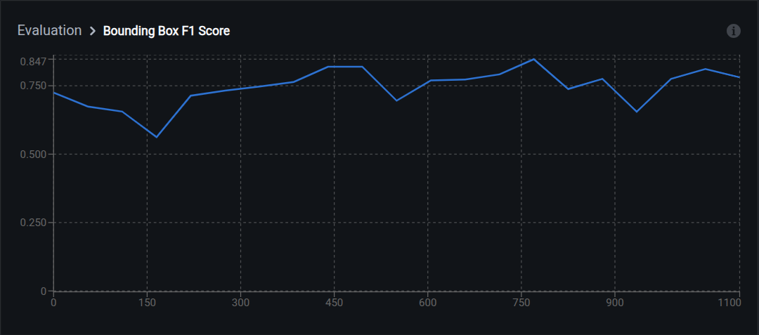
Range: 0.0 (worst) to 1.0 (perfect)

Interpretation:

• 0.90–1.00: Excellent detection accuracy
• 0.75–0.89: Good for most use cases
• 0.60–0.74: Acceptable for initial models; consider improvements
• Below 0.60: Needs significant improvement

How it works: F1 is the harmonic mean of precision and recall. The formula is F1 = 2 x (Precision x Recall) / (Precision + Recall). The harmonic mean ensures both precision and recall must be high for a high F1. Unlike arithmetic mean, it penalizes extreme imbalances between the two values.

Average IoU

IoU measures overlap between two rectangles: the predicted box and the correct box. The overlapping area divided by the total area covered by both boxes. An IoU of 0.5 means 50% overlap; 0.8 means 80% overlap.

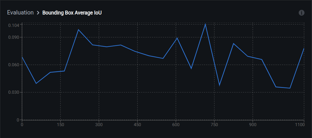
Range: 0.0 (no overlap) to 1.0 (perfect overlap)

Interpretation:

• 0.80–1.00: Tight bounding boxes
• 0.60–0.79: Good localization
• 0.50–0.59: Acceptable (standard detection threshold)
• Below 0.50: Poor localization; boxes are too loose or misaligned

How it works: IoU (Intersection over Union) measures overlap between predicted and ground truth boxes. The formula is IoU = Area of Overlap / Area of Union.

Standard thresholds used in the field:

• IoU ≥ 0.50: detection counts as correct (COCO standard)
• IoU ≥ 0.75: strict threshold
• IoU ≥ 0.95: strict (near pixel-perfect)

Precision

Precision measures how many of the model's predicted boxes are correct. A model with high precision rarely draws false boxes.

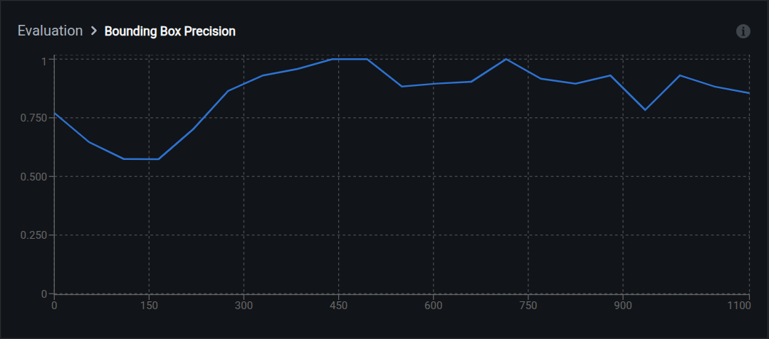
Range: 0.0 (all wrong) to 1.0 (all correct)

Interpretation:

• High precision (0.90+): Few false positives; predictions are reliable
• Low precision (below 0.70): Many false alarms; model over-detects

How it works: The formula is Precision = True Positives / (True Positives + False Positives).

Example: Model predicts 100 boxes, 85 correctly match ground truth, 15 are false alarms. Precision = 85/100 = 0.85.

Trade-off: Increasing precision often decreases recall.

Recall

Recall measures how many of the real objects the model found. A model with high recall misses few objects.

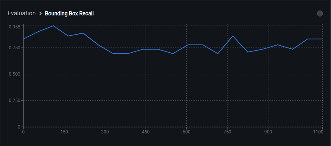
Range: 0.0 (missed everything) to 1.0 (found everything)

Interpretation:

• High recall (0.90+): Few missed detections
• Low recall (below 0.70): Many missed objects; model under-detects

How it works: The formula is Recall = True Positives / (True Positives + False Negatives).

Example: Ground truth contains 120 objects, model correctly detects 100, misses 20. Recall = 100/120 = 0.833.

Trade-off: Increasing recall often decreases precision. Adjusting the confidence threshold moves along the precision-recall curve: higher threshold gives higher precision and lower recall; lower threshold gives higher recall and lower precision.

Text generation metrics

These metrics apply to visual question answering tasks and evaluate how well generated text matches expected answers.

BLEU

BLEU compares word-for-word overlap between generated text and reference answers. "The car is red" vs "The red automobile" scores poorly even though they mean the same thing, because BLEU only checks exact n-gram matches.

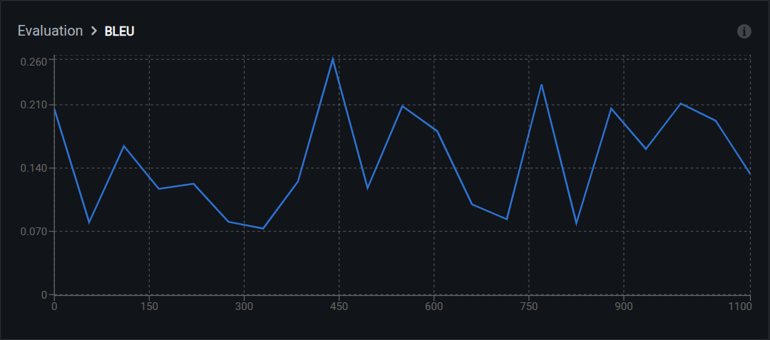
Range: 0.0 (no match) to 1.0 (perfect match)

Interpretation:

• 0.50–1.00: High-quality text generation with strong word overlap
• 0.30–0.49: Moderate quality; captures key concepts
• 0.10–0.29: Low overlap; answers may be semantically correct but worded differently
• Below 0.10: Poor text generation

Limitation: Does not capture semantic similarity. Synonyms or rephrasing lower the score even if the meaning is correct. Use BERTScore alongside BLEU for a fuller picture.

BERTScore

BERTScore uses a language model to compare meaning rather than exact words. "Car" and "automobile" score high because they mean the same thing. This makes it more reliable than BLEU for VQA evaluation where multiple phrasings are valid.

Components:

• BERTScore Recall: How much of the reference answer's meaning appears in predictions

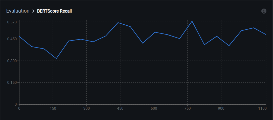
• BERTScore Precision: How much of the prediction's meaning matches the reference

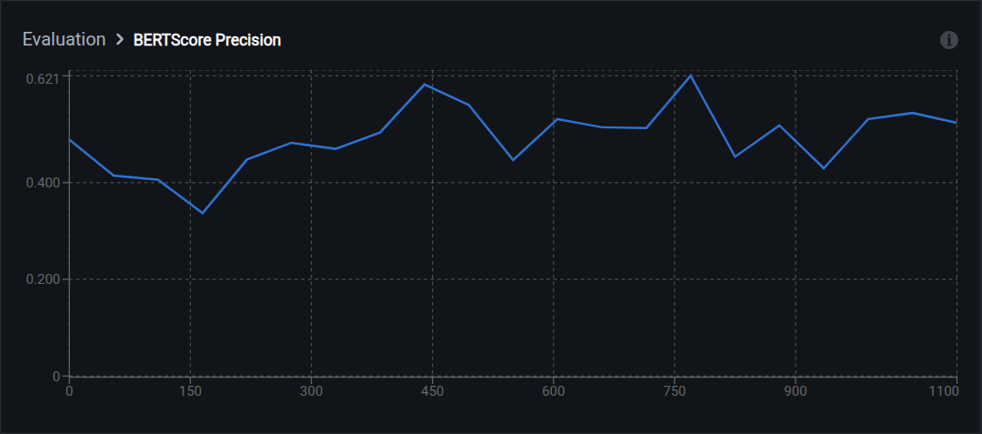
• BERTScore F1: Balanced combination of recall and precision

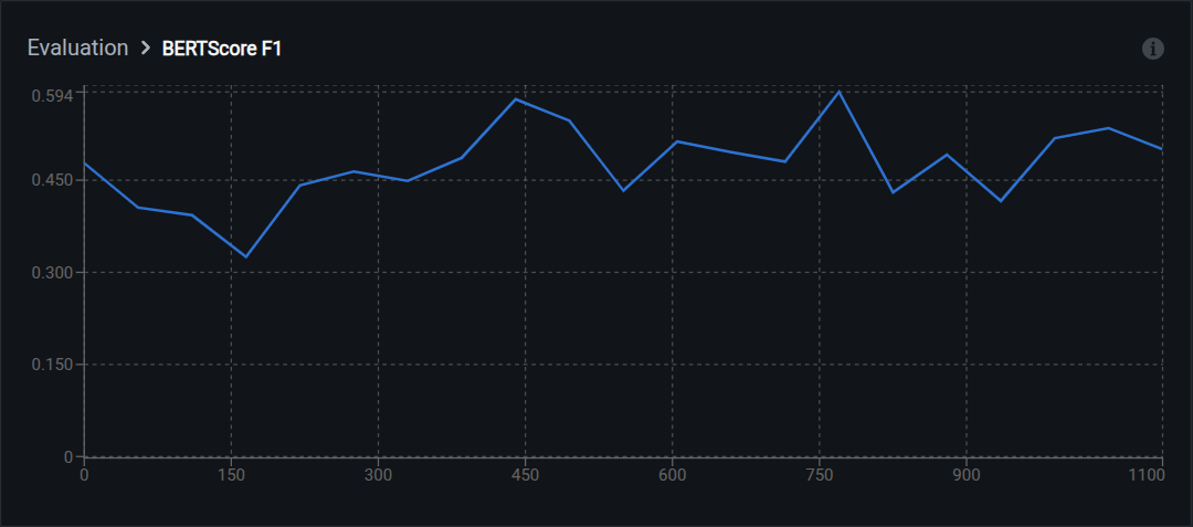
Range: 0.0 (no similarity) to 1.0 (identical meaning)

Interpretation:

• 0.90–1.00: Excellent semantic match
• 0.80–0.89: Good semantic similarity
• 0.70–0.79: Moderate; captures main concepts
• Below 0.70: Poor semantic alignment

Advantage over BLEU: Handles paraphrasing, synonyms, and different sentence structures. For example, "The vehicle has damage" and "The car is damaged" score low on BLEU but high on BERTScore because the embeddings recognize that the meanings are equivalent.

METEOR

METEOR measures text similarity considering synonyms, stemming, and word order. It sits between BLEU (exact match only) and BERTScore (full semantic comparison).

Range: 0.0 (no match) to 1.0 (perfect match)

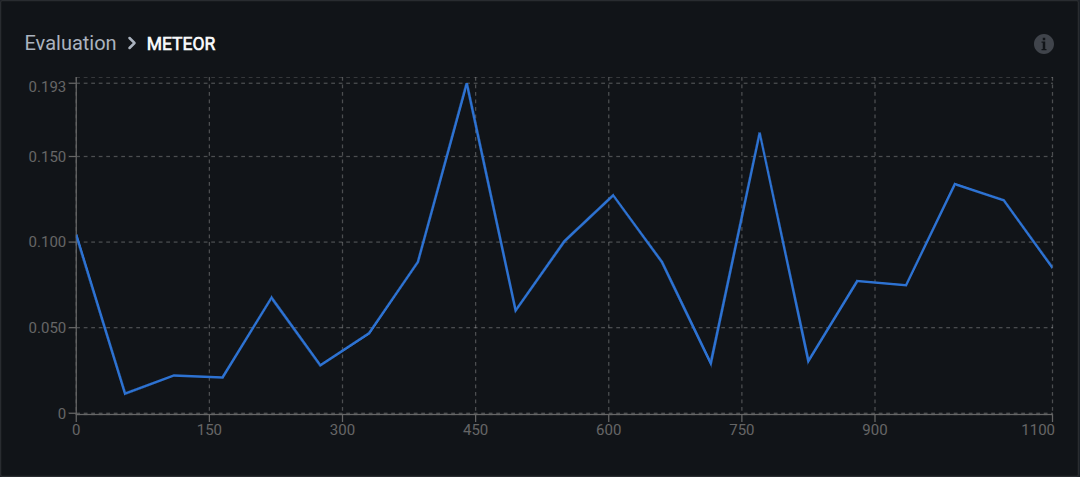
Interpretation:

• 0.60–1.00: Excellent quality with semantic understanding
• 0.40–0.59: Good quality; captures meaning with different wording
• 0.20–0.39: Acceptable; partial semantic match
• Below 0.20: Poor answer quality

Matching strategies used: exact word matches, stem matches (running = run), synonym matches (car = automobile), and paraphrase matches.

ROUGE

ROUGE measures overlap of n-grams, word sequences, and sentence structures. It is recall-oriented, meaning it focuses on how much of the reference content appears in the generated text rather than how precise the generation is.

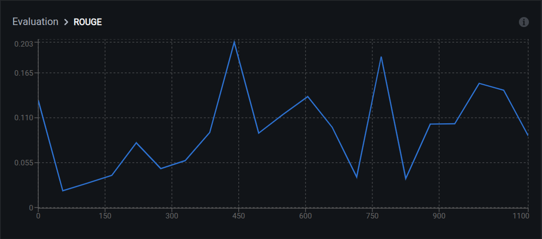
Variants:

• ROUGE-1: Unigram (single word) overlap
• ROUGE-2: Bigram (two-word sequence) overlap
• ROUGE-L: Longest common subsequence

Interpretation:

• 0.50–1.00: High content overlap; answers are thorough
• 0.30–0.49: Moderate overlap; key information present
• 0.15–0.29: Low overlap; may miss important details
• Below 0.15: Poor content coverage

Best for: Visual question answering tasks where answer completeness matters, such as detailed descriptions or multi-part questions.

Hyperparameters

The hyperparameters section displays key training settings for the run.

Learning rate controls how quickly the model updates during training. Two values are shown:

• Initial learning rate: The starting value at the beginning of training
• Final learning rate: The value at the end of training (may decrease via learning rate scheduling)

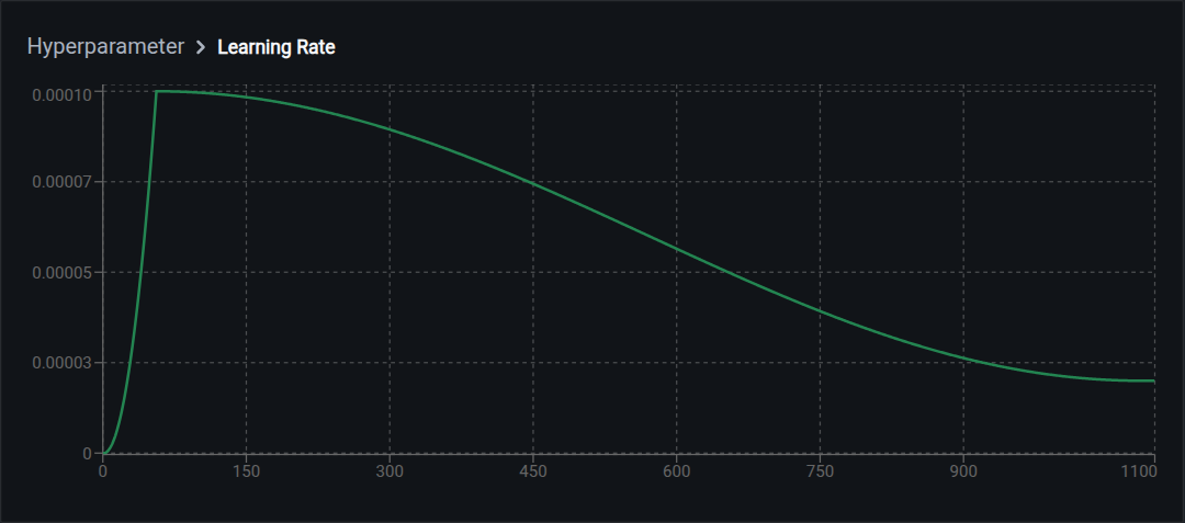
Typical ranges:

• LoRA training: 1e-4 to 5e-4
• Full fine-tuning: 1e-5 to 1e-4

For the full training configuration (batch size, epochs, optimizer), check the run configuration or the Logs tab.

Comparing runs

Systematic comparison helps identify which configuration changes improve performance. The key practice is changing one variable at a time.

Less useful approach: Change model, learning rate, and batch size all at once between runs. You cannot tell which change caused any improvement or regression.

Better approach: Keep all variables fixed except one per run. Example:

• Run 1 (baseline): Model A, learning rate 3e-4, batch size 8
• Run 2: Model B, learning rate 3e-4, batch size 8 (only model changed)
• Run 3: Model B, learning rate 1e-4, batch size 8 (only learning rate changed)

Document final loss, F1, and BLEU scores for each run. Use Advanced Evaluation to compare predictions on the same validation images across runs.

Understanding overfitting

Overfitting occurs when a model memorizes training data instead of learning patterns that generalize to new images. The model performs well on training data but poorly on validation data.

The main signal is a widening gap between your orange (training) and blue (validation) loss curves. Training loss keeps improving while validation loss plateaus or gets worse.

Other signs:

• Evaluation metrics improve on training checkpoints but degrade on later ones
• Model predicts training images accurately but misses validation examples
• Performance drops on images with different lighting, angles, or backgrounds than training data

How to address overfitting

Do this with the Vi SDK

import vi

client = vi.Client(
    secret_key="your-secret-key",
    organization_id="your-organization-id"
)

models = client.models.list("your-run-id")
for model in models.items:
    if model.spec.evaluation_metrics:
        for metric, value in model.spec.evaluation_metrics.items():
            print(f"{metric}: {value}")

For more details, see the full SDK reference.

Next steps