Metrics
Analyze quantitative performance measurements including loss curves, evaluation metrics, and hyperparameters.
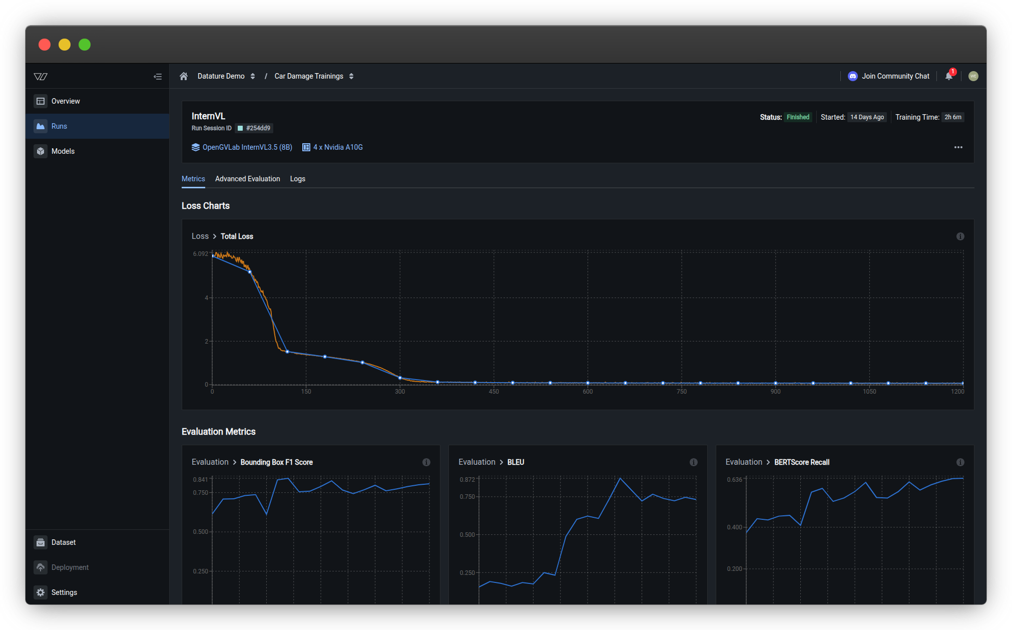
The Metrics tab provides quantitative performance measurements tracked throughout training. Use these metrics to assess model quality, identify overfitting, and compare runs.
Prerequisites
- A completed training run or active run with metrics
- Understanding of loss functions and evaluation metrics
- Familiarity with model evaluation concepts
- Access to training project with runs
Access metricsOpen any completed training run and click the Metrics tab to view loss curves, evaluation metrics, and hyperparameters.
Loss charts
Loss measures how far the model's predictions are from the ground truth. Lower loss indicates better alignment with training data.
Understanding chart colors
- Orange curves — Training losses recorded at every training step (more granular)
- Blue curves — Validation losses and metrics recorded at every evaluation interval (less granular)
Total loss
The primary training metric showing overall model error over time.
What to look for:
- ✅ Steady decrease — Model is learning successfully
- ✅ Plateau at low value — Model has converged to optimal performance
- ⚠️ Sudden spikes — May indicate learning rate issues or data quality problems
- ⚠️ No decrease — Model isn't learning; check hyperparameters or dataset quality
Understanding loss values
What do loss numbers mean?
Loss values depend on your model architecture and task:
- Starting loss — Typically 2.0-6.0 for untrained models
- Good final loss — 0.5-1.5 for well-trained models
- Excellent final loss — Below 0.5 for high-quality datasets
Important: Compare loss across runs for the same model and dataset. Different architectures have different loss scales, so absolute values aren't directly comparable.
Common loss curve patterns
Normal training:
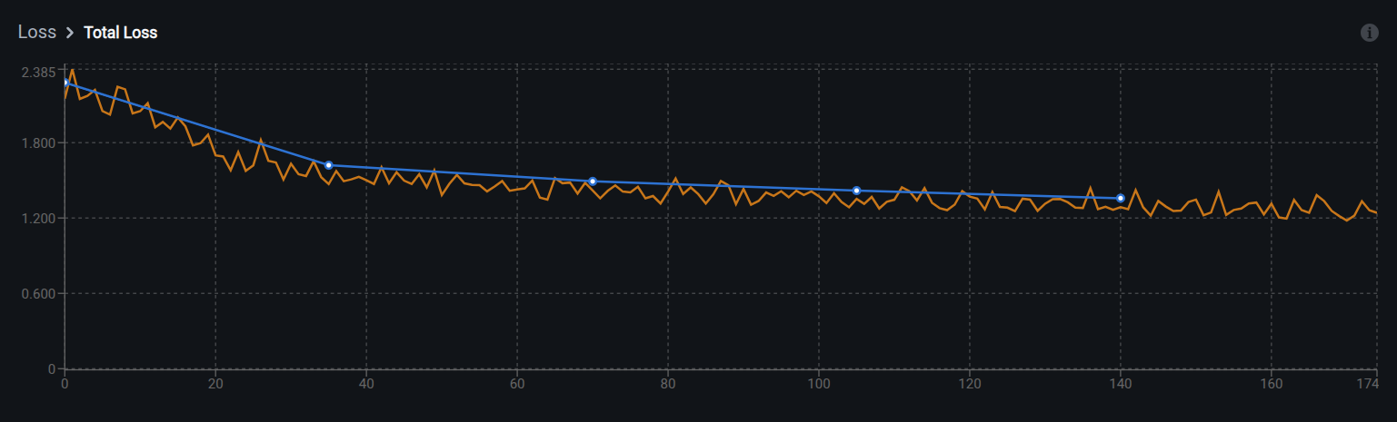
What to expect: Both orange (training) and blue (validation) curves show rapid decrease initially, then gradual plateau at a low value. The curves should stay relatively close to each other, indicating the model is learning generalizable patterns.
Underfitting:
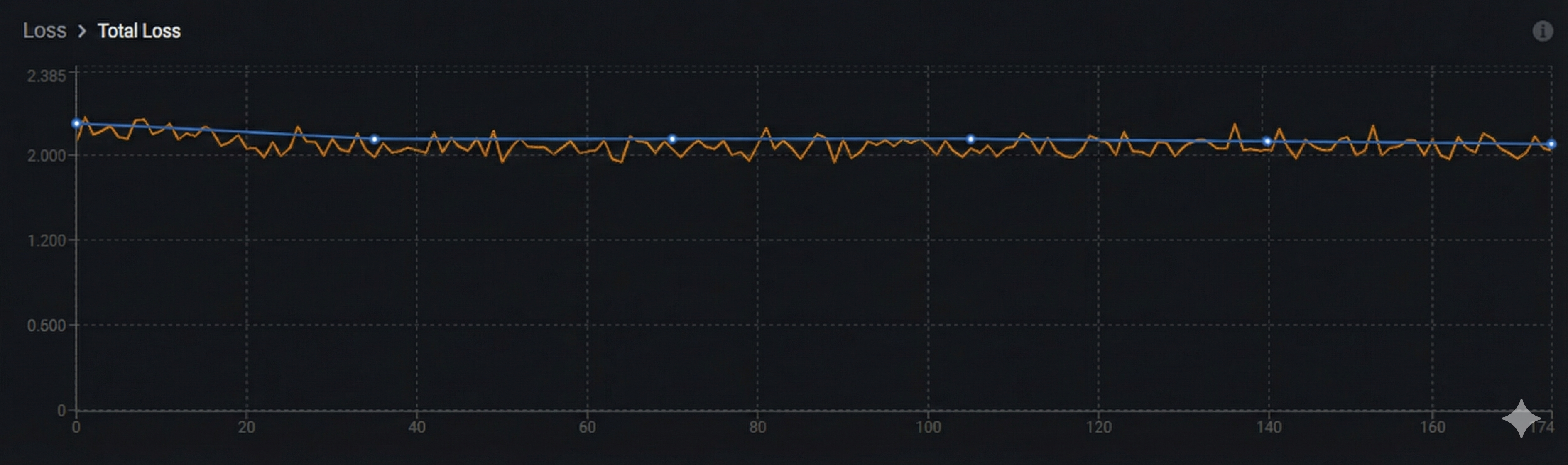
Key indicator: Both orange (training) and blue (validation) curves show minimal decrease and remain relatively flat. The model hasn't learned enough from the data.
What's happening:
- Both curves plateau at high loss values or show minimal improvement
- Little to no decrease over time
- Model is too simple, learning rate is too low, or training is insufficient
Solutions: Train longer, use a larger model, increase learning rate, or check data quality.
Overfitting:
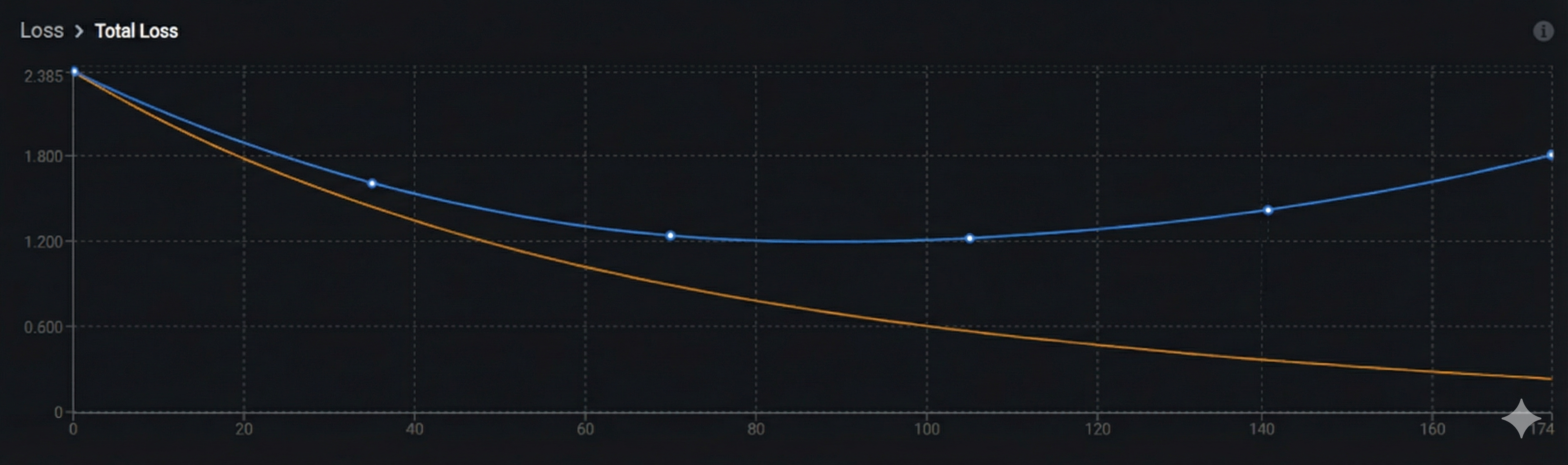
Key indicator: Orange (training) loss continues decreasing while blue (validation) loss plateaus or starts increasing. The gap between the two curves widens over time.
What's happening:
-
Training loss keeps improving but validation loss stops improving or gets worse
-
Model is memorizing training data instead of learning generalizable patterns
-
Occurs with extended training, overly complex models, or insufficient data
Solutions: Stop training earlier (use early stopping), reduce model complexity, add regularization, or increase dataset size.
Evaluation metrics
Evaluation metrics measure how well your model performs on specific tasks. Available metrics depend on your task type:
- Bounding box metrics — For phrase grounding tasks
- Text generation metrics — For VQA tasks
Bounding box metrics
For phrase grounding tasks, these metrics evaluate object detection quality:
Bounding Box F1 Score
What it measures: Overall detection accuracy balancing precision and recall.
Range: 0.0 (worst) to 1.0 (perfect)
Interpretation:
- 0.90-1.00 — Excellent detection accuracy
- 0.75-0.89 — Good performance for most use cases
- 0.60-0.74 — Acceptable for initial models; consider improvements
- Below 0.60 — Needs significant improvement
When to prioritize: General use cases where you want balanced false positive and false negative rates.
How it's calculated:
F1 Score is the harmonic mean of precision and recall:
F1 = 2 × (Precision × Recall) / (Precision + Recall)Where:
- Precision = True Positives / (True Positives + False Positives)
- Recall = True Positives / (True Positives + False Negatives)
The harmonic mean ensures that both precision and recall must be high for a high F1 score. Unlike arithmetic mean, it penalizes extreme imbalances between precision and recall.
Learn more:
Bounding Box Average IoU
What it measures: How well predicted bounding boxes overlap with ground truth boxes.
Range: 0.0 (no overlap) to 1.0 (perfect overlap)
Interpretation:
- 0.80-1.00 — Very tight bounding boxes
- 0.60-0.79 — Good localization
- 0.50-0.59 — Acceptable (standard detection threshold)
- Below 0.50 — Poor localization; boxes are too loose or misaligned
When to prioritize: When precise object localization is critical (e.g., robotic picking, measurement tasks).
How it's calculated:
IoU (Intersection over Union) measures the overlap between predicted and ground truth boxes:
IoU = Area of Overlap / Area of UnionVisual representation:
Ground Truth Box: [====]
Predicted Box:      [====]
Overlap:            [==]
Union:          [======]

IoU = Area of [==] / Area of [======]
Calculation steps:
- Find intersection area (where boxes overlap)
- Find union area (combined coverage of both boxes)
- Divide intersection by union
- Average across all detected objects
Standard thresholds:
- IoU ≥ 0.50 — Detection counts as "correct" (COCO standard)
- IoU ≥ 0.75 — Strict detection threshold
- IoU ≥ 0.95 — Very strict (pixel-perfect requirement)
Learn more:
Bounding Box Precision
What it measures: Of all predicted bounding boxes, what percentage are correct?
Range: 0.0 (all wrong) to 1.0 (all correct)
Interpretation:
- High precision (0.90+) — Few false positives; predictions are reliable
- Low precision (<0.70) — Many false alarms; model over-detects
When to prioritize:
- Quality control where false alarms are costly
- Applications where you need high confidence in every detection
- When downstream systems can't handle false positives
Trade-off: Increasing precision often decreases recall.
How it's calculated:
Precision measures the accuracy of positive predictions:
Precision = True Positives / (True Positives + False Positives)Or equivalently:
Precision = Correct Detections / All DetectionsExample:
- Model predicts 100 bounding boxes
- 85 boxes correctly match ground truth objects (True Positives)
- 15 boxes are false alarms on background/wrong objects (False Positives)
- Precision = 85 / (85 + 15) = 85 / 100 = 0.85 or 85%
What affects precision:
- Lower confidence threshold → More detections → Lower precision (more false positives)
- Higher confidence threshold → Fewer detections → Higher precision (fewer false positives)
Learn more:
Bounding Box Recall
What it measures: Of all actual objects, what percentage did the model find?
Range: 0.0 (missed everything) to 1.0 (found everything)
Interpretation:
- High recall (0.90+) — Few missed detections; model finds nearly everything
- Low recall (<0.70) — Many missed objects; model under-detects
When to prioritize:
- Safety-critical applications where missing objects is dangerous
- Inventory or counting tasks where completeness matters
- When false negatives are more costly than false positives
Trade-off: Increasing recall often decreases precision.
How it's calculated:
Recall measures the completeness of detections:
Recall = True Positives / (True Positives + False Negatives)Or equivalently:
Recall = Detected Objects / All Ground Truth ObjectsExample:
- Ground truth contains 120 objects
- Model detects 100 of them correctly (True Positives)
- Model misses 20 objects (False Negatives)
- Recall = 100 / (100 + 20) = 100 / 120 = 0.833 or 83.3%
What affects recall:
- Lower confidence threshold → More detections → Higher recall (fewer missed objects)
- Higher confidence threshold → Fewer detections → Lower recall (more missed objects)
- Model capacity → Larger models often achieve higher recall
Recall vs. Precision trade-off:
Adjusting the confidence threshold moves along the precision-recall curve:
- High threshold → High precision, low recall (conservative predictions)
- Low threshold → Low precision, high recall (aggressive predictions)
- Optimal threshold → Balanced F1 score
Learn more:
Text generation metrics
For VQA tasks, these metrics evaluate response quality:
BLEU (Bilingual Evaluation Understudy)
What it measures: N-gram overlap between generated text and reference answers.
Range: 0.0 (no match) to 1.0 (perfect match)
Interpretation:
- 0.50-1.00 — High-quality text generation with strong word overlap
- 0.30-0.49 — Moderate quality; captures key concepts
- 0.10-0.29 — Low overlap; answers may be semantically correct but worded differently
- Below 0.10 — Poor text generation
Strengths: Good for tasks with specific terminology or structured answers.
Limitations: Doesn't capture semantic similarity—synonyms or rephrasing lower scores even if meaning is correct.
How it's calculated:
BLEU measures n-gram precision (word sequence overlap) with a brevity penalty:
BLEU = BP × exp(Σ wₙ × log(pₙ))Where:
- pₙ = Precision of n-grams (unigrams, bigrams, trigrams, 4-grams)
- wₙ = Weight for each n-gram (typically uniform: 0.25 each)
- BP = Brevity penalty (penalizes outputs shorter than reference)
Simplified calculation:
-
Count matching n-grams:
- Reference: "The car is red"
- Prediction: "The red car"
- Matching unigrams: "The", "red", "car" (3/3)
- Matching bigrams: None (0/2)
-
Calculate precision for each n-gram level
-
Apply brevity penalty if prediction is too short
-
Geometric mean of n-gram precisions
Example:
Reference: "There are three defects visible"
Prediction: "Three defects are visible"

Unigram precision: 4/4 = 1.0 (all words match)
Bigram precision: 2/3 = 0.67 ("defects are", "are visible")
Trigram precision: 1/2 = 0.5 ("are visible")
4-gram precision: 0/1 = 0

BLEU ≈ 0.46 (moderate score due to different word order)
Learn more:
BERTScore (Recall, Precision, F1)
What it measures: Semantic similarity using contextual embeddings (not just word overlap).
Components:
- BERTScore Recall — How much of the reference answer's meaning appears in predictions
- BERTScore Precision — How much of the prediction's meaning matches the reference
- BERTScore F1 — Balanced combination of recall and precision
Range: 0.0 (no similarity) to 1.0 (identical meaning)
Interpretation:
- 0.90-1.00 — Excellent semantic match
- 0.80-0.89 — Good semantic similarity
- 0.70-0.79 — Moderate similarity; captures main concepts
- Below 0.70 — Poor semantic alignment
Strengths: Handles paraphrasing, synonyms, and different sentence structures.
When to use: VQA tasks where multiple valid phrasings exist for the same answer.
How it's calculated:
BERTScore uses BERT embeddings to measure semantic similarity between texts:
Step 1: Generate contextual embeddings
Each word in both reference and prediction is encoded using a pre-trained language model (BERT) to capture meaning in context.
Step 2: Compute token similarity
Calculate cosine similarity between each token embedding in the prediction and reference:
similarity(t_pred, t_ref) = cos(embedding_pred, embedding_ref)Step 3: Match tokens
For each token, find the most similar token in the other text using maximum cosine similarity.
Step 4: Calculate precision, recall, F1
BERTScore Precision = Σ max_similarity(pred_token, ref_tokens) / |prediction|
BERTScore Recall = Σ max_similarity(ref_token, pred_tokens) / |reference|
BERTScore F1 = 2 × (Precision × Recall) / (Precision + Recall)
Example:
Reference: "The vehicle has damage"
Prediction: "The car is damaged"

Traditional word overlap: Low (only "the" matches exactly)
BERTScore: High (embeddings recognize "vehicle"≈"car", "damage"≈"damaged")
Why it's better than BLEU:
- Semantic understanding: Recognizes synonyms ("car" = "vehicle")
- Contextual meaning: "bank" (river) vs "bank" (financial) handled correctly
- Flexible matching: Different word forms, paraphrasing captured
Learn more:
METEOR (Metric for Evaluation of Translation with Explicit Ordering)
What it measures: Text similarity considering synonyms, stemming, and word order.
Range: 0.0 (no match) to 1.0 (perfect match)
Interpretation:
- 0.60-1.00 — Excellent answer quality with semantic understanding
- 0.40-0.59 — Good quality; captures meaning with different wording
- 0.20-0.39 — Acceptable; partial semantic match
- Below 0.20 — Poor answer quality
Strengths:
- Recognizes synonyms (e.g., "car" and "automobile")
- Handles different word forms (e.g., "running" and "run")
- Rewards word order similarity
When to use: Tasks requiring flexible language evaluation beyond exact word matching.
How it's calculated:
METEOR computes alignment between reference and prediction text considering multiple matching strategies:
Step 1: Alignment (find matches using multiple strategies)
Match words between reference and prediction using:
- Exact match: Words are identical ("car" = "car")
- Stem match: Same root form ("running" = "run")
- Synonym match: Words from same synset ("car" = "automobile")
- Paraphrase match: Semantically equivalent phrases
Step 2: Calculate base score
P = matches / words_in_prediction (precision)
R = matches / words_in_reference (recall)

F-mean = (P × R) / (α × P + (1-α) × R)
where α is typically 0.9 (favoring recall slightly)
Step 3: Apply fragmentation penalty
Penalizes non-contiguous matches (words matched in different order):
Penalty = γ × (chunks / matches)^βWhere:
- chunks = Number of contiguous match segments
- γ, β = Tuning parameters (typically γ=0.5, β=3)
Step 4: Final score
METEOR = F-mean × (1 - Penalty)Example:
Reference: "The damaged car needs repair"
Prediction: "The car is damaged and requires fixing"

Exact matches: "The", "car" (2)
Stem matches: "damaged" = "damaged" (1)
Synonym matches: "repair" ≈ "fixing" (1)

Total matches: 4
Chunks: 3 (non-contiguous: "The car", "damaged", "fixing")
Penalty applied for fragmentation

METEOR ≈ 0.52
Learn more:
ROUGE (Recall-Oriented Understudy for Gisting Evaluation)
What it measures: Overlap of n-grams, word sequences, and sentence structures.
Variants displayed:
- ROUGE-1 — Unigram (single word) overlap
- ROUGE-2 — Bigram (two-word sequence) overlap
- ROUGE-L — Longest common subsequence
Range: 0.0 (no overlap) to 1.0 (complete overlap)
Interpretation:
- 0.50-1.00 — High content overlap; answers are comprehensive
- 0.30-0.49 — Moderate overlap; key information present
- 0.15-0.29 — Low overlap; may miss important details
- Below 0.15 — Very poor content coverage
Strengths: Good for evaluating answer completeness and content coverage.
When to use: VQA tasks where comprehensive answers matter (e.g., detailed descriptions, multi-part questions).
How it's calculated:
ROUGE measures recall-oriented n-gram overlap (focuses on coverage rather than precision):
ROUGE-1 (Unigram overlap):
ROUGE-1 = Count of overlapping words / Total words in referenceExample:
Reference: "The car has front damage"  (5 words)
Prediction: "Front and rear car damage visible"  (6 words)

Overlapping words: "car", "front", "damage" (3)
ROUGE-1 = 3 / 5 = 0.60
ROUGE-2 (Bigram overlap):
ROUGE-2 = Count of overlapping bigrams / Total bigrams in referenceExample:
Reference: "The car has front damage"
Bigrams: "The car", "car has", "has front", "front damage" (4)

Prediction: "Front car damage is visible"
Overlapping bigrams: "front damage" (1)

ROUGE-2 = 1 / 4 = 0.25
ROUGE-L (Longest Common Subsequence):
Finds the longest sequence of words that appear in both texts (order matters, but words don't need to be consecutive):
ROUGE-L = LCS(reference, prediction) / length(reference)Example:
Reference: "The red car has damage"
Prediction: "The car is red with visible damage"

LCS: "The", "red", "car", "damage" (4 words, maintaining order)
ROUGE-L = 4 / 5 = 0.80
Why "Recall-Oriented"?
ROUGE emphasizes recall (coverage of reference content) over precision:
- Measures: What percentage of reference content appears in prediction?
- Good for: Summaries, descriptions where completeness matters
- Less sensitive to: Extra content in predictions
Learn more:
Hyperparameters
The hyperparameters section displays key training settings used for this run.
Learning rate
What it is: Controls how quickly the model updates during training.
Displayed values:
- Initial learning rate — Starting value at beginning of training
- Final learning rate — Value at end of training (may decrease via learning rate scheduling)
Typical ranges:
- LoRA training: 1e-4 to 5e-4 (0.0001 to 0.0005)
- Full fine-tuning: 1e-5 to 1e-4 (0.00001 to 0.0001)
View all hyperparametersTo see complete training configuration including batch size, epochs, and optimizer settings, view the run configuration or check the Logs tab.
Compare multiple runs
Systematic comparison helps identify which configuration changes improve performance.
Comparison workflow
Compare metrics across runs
Create a comparison table:
| Run | Model | Learning Rate | Final Loss | Bbox F1 | BLEU |
|---|---|---|---|---|---|
| Run 1 | Qwen2.5-VL 2B | 3e-4 | 0.82 | 0.78 | 0.45 |
| Run 2 | Qwen2.5-VL 7B | 3e-4 | 0.64 | 0.85 | 0.52 |
| Run 3 | Qwen2.5-VL 7B | 1e-4 | 0.58 | 0.88 | 0.56 |
Analysis:
- Run 1 → Run 2: Larger model improves all metrics
- Run 2 → Run 3: Lower learning rate further improves convergence
Conclusion: Qwen2.5-VL 7B with learning rate 1e-4 is optimal configuration.
Compare visual predictions
For each configuration:
- Open Advanced Evaluation for the run
- Navigate to the same evaluation specimen across runs
- Compare predictions side-by-side (manually or via screenshots)
What to compare:
- Bounding box quality — Tightness, completeness, false positives
- Text generation — Accuracy, completeness, formatting
- Consistency — Performance across different image types
- Edge case handling — Behavior on difficult examples
Document findings: Note which configuration handles specific scenarios better.
Systematic experimentation
Best practice: Change one variable at a time
❌ Bad approach:
- Run 1: Model A, learning rate 3e-4, batch size 8, epochs 3
- Run 2: Model B, learning rate 1e-4, batch size 16, epochs 5
Impossible to determine which change caused improvements
✅ Good approach:
- Run 1 (baseline): Model A, learning rate 3e-4, batch size 8, epochs 3
- Run 2: Model B, learning rate 3e-4, batch size 8, epochs 3 (only model changed)
- Run 3: Model B, learning rate 1e-4, batch size 8, epochs 3 (only learning rate changed)
- Run 4: Model B, learning rate 1e-4, batch size 16, epochs 3 (only batch size changed)
Clear cause-and-effect relationships
Understanding overfitting
Overfitting occurs when a model memorizes training data instead of learning general patterns. The model performs well on training data but poorly on new, unseen images.
Signs of overfitting
Watch for diverging training and validation performance. The most reliable indicator is when your orange curves (training) keep improving while blue curves (validation) plateau or degrade.
Loss curve indicators
Training loss vs. validation loss:
Remember: Orange curves = training loss (granular), Blue curves = validation loss (evaluation intervals)
✅ Healthy training:
Both orange (training) and blue (validation) curves decrease together. Validation stays close to training loss throughout the entire training process, indicating the model is learning generalizable patterns rather than memorizing.
⚠️ Problematic training (overfitting):
Key indicator: Orange (training) loss continues decreasing while blue (validation) loss plateaus or starts increasing. The gap between the two curves widens over time.
What's happening:
-
Training loss keeps improving but validation loss stops improving or gets worse
-
Model is memorizing training data instead of learning generalizable patterns
-
Occurs with extended training, overly complex models, or insufficient data
Solutions: Stop training earlier (use early stopping), reduce model complexity, add regularization, or increase dataset size.
Metric degradation
Check evaluation metrics over checkpoints:
⚠️ Overfitting signs:
- Metrics improve on training set but degrade on validation set
- Metrics peak at early checkpoint, then decline
- Large gap between train and validation performance
Example:
| Checkpoint | Train F1 | Validation F1 | Status |
|---|---|---|---|
| Step 500 | 0.75 | 0.72 | ✅ Healthy |
| Step 1000 | 0.85 | 0.80 | ✅ Healthy |
| Step 1500 | 0.92 | 0.78 | ⚠️ Overfitting |
| Step 2000 | 0.97 | 0.74 | ❌ Severe overfitting |
Visual prediction issues
⚠️ Overfitting behaviors:
- Model performs perfectly on training images but poorly on validation images
- Predictions are overly specific to training examples (e.g., only detects objects in exact poses seen during training)
- Model fails on slight variations of training examples
- Performance degrades on images with different lighting, angles, or contexts than training data
Prevent and fix overfitting
Add more training data
Most effective solution:
- Increase dataset size (aim for 2× current size)
- Add diverse examples covering different:
- Lighting conditions
- Object orientations and poses
- Backgrounds and contexts
- Image quality and resolutions
Train for fewer epochs
Early stopping:
- Monitor validation metrics during training
- Identify checkpoint where validation performance peaks
- Kill the run at or shortly after peak
- Use that checkpoint for deployment
Automatic early stopping:
Configure checkpoint frequency to save more checkpoints for granular stopping.
Adjust hyperparameters
Reduce model capacity:
- Use smaller model architecture (e.g., 2B instead of 7B)
- Lower learning rate
- Reduce training epochs
Increase regularization:
- Add dropout (if supported by architecture)
- Use stronger weight decay
Improve data quality
Quality over quantity:
- Fix annotation errors and inconsistencies
- Remove duplicate or near-duplicate images
- Balance class distribution
- Add hard negatives (challenging examples)
Related resources
- Evaluate a model — Complete guide to model evaluation
- Monitor a run — Track training progress in real-time
- Advanced evaluation — Visual predictions and detailed analysis
- Logs — View training logs and debug issues
- Train a model — Complete training guide
- Configure your model — Select model architecture and hyperparameters
- Manage runs — Kill or delete runs
- Resource usage — Understand GPU costs and training time
- Configure training settings — Set checkpoint strategy and evaluation
- Phrase grounding — Understand object detection metrics
- Visual question answering — Understand text generation metrics
- Quickstart — End-to-end training tutorial
Need help?
We're here to support your VLMOps journey. Reach out through any of these channels:
Updated 3 months ago